This post introduces a series I intend to write, exploring using Variational Inference to massively speed up running complex survey estimation models like variants of Multilevel Regression and Poststratification while aiming to keep approximation error from completely ruining the model.

The rough plan for the series is as follows:

(This post) Introducing the Problem- Why is VI useful, why VI can produce spherical cows
How far does iteration on classic VI algorithms like mean-field and full-rank get us?
Some theory on why posterior approximation with VI can be so poor
Seeing if some more sophisticated techniques like normalizing flows help

Motivation for series

I learn well by explaining things to others, and I’ve been particularly excited to learn about variational inference and ways to improve it over the past few months. There are lots of Bayesian models I would like to fit, especially in my political work, that I would categorize as being incredibly useful, but on the edge of practically acceptable run times. For example, the somewhat but not particularly complex model I’ll use as a running example for the series takes ~8 hours to fit on 60k observations.

Having a model run overnight or for a full work day can be fine sometimes, but what if there is a more urgent need for the results? What if we need to iterate to find the “right” model? What if the predictions from this model need to feed into a later one? How constrained do we feel about adding just a little bit more complexity to the model, or increasing our N size just a bit more?

If we can get VI to fit well, we can make complex Bayesian models a lot more practical to use in a wider variety of scenarios, and maybe even extend the complexity of what we can build given time and resource constraints.

Spherical Cow Sadness

I’ve got that…

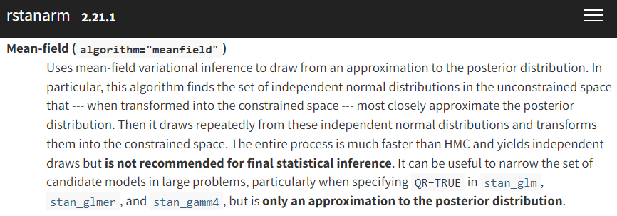
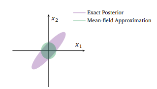
If VI can make Bayesian inference much faster, what’s the catch? The above two images encapsulate the problem pretty well. First, as the left screenshot from rstanarm’s documentation shows, variational inference requires a (bold text warning requiring) set of approximating distribution choices in order to be tractable to optimize. On the right, in their survey paper on VI, Blei et al. (2018) are showing one of the potential posterior distorting consequences of our choice to approximate.

So stepping back for a second, we’ve taken a problem for which there’s usually no closed form solution (Bayesian inference), where even the best approximation algorithm we can usually use (MCMC) isn’t always enough for valid inference without very careful validation and tinkering. Then we decided our approximation could do with being more approximate.

That was perhaps an overly bleak description, but it should give some intuition why this is a hard problem. We want to choose some method of approximating our posterior such that it is amenable to optimization-based solving instead of requiring sampling, but not trade away our ability to correctly understand the full complexity of the posterior distribution¹.

Introducing MRP and our running example

Introducing MRP

While I’m mostly focused on the way we choose to actually fit a given model with this series, here’s a super quick review of the intuition in building a MRP model. If you want a more complete introduction, Kastellec’s MRP Primer is a great starting point, as are the case studies I link a bit later.

MRP casts estimation of a population quantity of interest \theta as a prediction problem. That is, instead of the more traditional approach of building simple raked weights and using weighted estimators, MRP leans more heavily on modeling and then poststratification to make the estimates representative.

To sketch out the steps-

Either gather or run a survey or collection of surveys that collect both information on the outcome of interest, y, and a set of demographic and geographic predictors, \left(X_{1}, X_{2}, X_{3}, \ldots, X_{m}\right).
Build a poststratification table, with population counts or estimated population counts N_{j} for each possible combination of the features gathered above. Each possible combination j is called a cell, one of J possible cells. For example, if we poststratified only on state, there would be J=51 (with DC) total cells; in practice, J is often several thousand.
Build a model, usually a Bayesian multilevel regression, to predict y using the demographic characteristic from the survey or set of surveys, estimating model parameters along the way.
Estimate y for each cell in the poststratification table, using the model built on the sample.
Aggregate the cells to the population of interest, weighting by the N_{j}’s to obtain population level estimates: \theta_{\mathrm{POP}}=\frac{\sum_{j \in J} N_{j} \theta_{j}}{\sum_{j \in J} N_{J}}

Why would we want to do this over building more typical survey weights? To the extent your new model has desirable properties like the ability to incorporate priors, can partially pool to manage rare subpopulations where you don’t have a lot of sample, and so on, you can get the benefits of that more efficient model through MRP. Raking in its simplest form is really just a linear model; we have plenty of methods that can do better. Outside of bayesian multilevel models which are the most common, there’s an increasing literature on using a wide variety of machine learning algorithms like BART² to do the estimation stage; Andrew Gelman calls this RRP.

Introducing the Running Example

Rather than reinvent the wheel, I’ll follow the lead of the excellent Multilevel Regression and Poststratification Case Studies by Lopez-Martin, Philips, and Gelman, and model survey binary responses from the 2018 CCES for the following question:

Allow employers to decline coverage of abortions in insurance plans (Support / Oppose)

From the CCES, we get information on each participant’s state, age, gender, ethnicity, and education level. Supplementing this individual level data, we also include region flags for each state, and Republican vote share in the 2016 election- these state level predictors have been shown to be critical for getting strong MRP estimates by Lax and Philips (2009) and others. and If you’d like deeper detail on the dataset itself, I’d refer you to this part MRP case study.

Using these, we setup the model for Pr(y_i = 1) the probability of supporting allowing employers to decline coverage of abortions in insurance plans as:

\begin{aligned} Pr(y_i = 1) =& logit^{-1}( \gamma^0 + \alpha_{\rm s[i]}^{\rm state} + \alpha_{\rm a[i]}^{\rm age} + \alpha_{\rm r[i]}^{\rm eth} + \alpha_{\rm e[i]}^{\rm educ} + \beta^{\rm male} \cdot {\rm Male}_{\rm i} \\ &+ \alpha_{\rm g[i], r[i]}^{\rm male.eth} + \alpha_{\rm e[i], a[i]}^{\rm educ.age} + \alpha_{\rm e[i], r[i]}^{\rm educ.eth} + \gamma^{\rm south} \cdot {\rm South}_{\rm s} \\ &+ \gamma^{\rm northcentral} \cdot {\rm NorthCentral}_{\rm s} + \gamma^{\rm west} \cdot {\rm West}_{\rm s} + \gamma^{\rm repvote} \cdot {\rm RepVote}_{\rm s}) \end{aligned}

Where we incorporate pretty much all of our predictors as varying intercepts to allow for pooling across demographic and geographic characteristics:

\alpha_{\rm a}^{\rm age}: The effect of subject i’s age on the probability of supporting the statement.
\alpha_{\rm r}^{\rm eth}: The effect of subject i’s ethnicity on the probability of supporting the statement.
\alpha_{\rm e}^{\rm educ}: The effect of subject i’s education on the probability of supporting the statement.
\alpha_{\rm s}^{\rm state}: The effect of subject i’s state on the probability of supporting the statement.
\beta^{\rm male}: The average effect of being male on the probability of supporting abortion. Note that it doesn’t really make much sense to model a two category³ factor as a varying intercept.
\alpha_{\rm e,r}^{\rm male.eth}, \alpha_{\rm e,r}^{\rm educ.age}, \alpha_{\rm e,r}^{\rm educ.eth}: Are several reasonable guesses at important interactions for this question. We could add many more two way, or even some three way interactions here, but this is enough for my testing here.
\gamma^{\rm south}, \gamma^{\rm northcentral}, \gamma^{\rm west},\gamma^{\rm repvote}: are the state level predictors which are not represented as varying intercepts. Following the case study, I use \gamma’s for the state level coefficients, keeping \beta’s for individual coefficients. Note that Northeast is the base region of the region factor here, so it doesn’t get it’s own coefficient.

Stepping back for a second, let’s describe the complexity of this model in more general terms. This certainly isn’t state of the art for MRP, and you could definitely add in things like a lot more interactions, some varying slopes, non-univariate prior and/or structured priors, or other elements to make this a more interesting model. That said, this is already clearly enough of a model to improve on simple raking in many cases, and it produces a nuanced enough posterior that we can feasibly imagine a bad approximation going all spherical cow shaped on us.

Why this dataset and this model for this series? The question we model itself isn’t super important- as long as we can expect some significant regional and demographic variation in the outcome we’ll be able to explore if VI smoothes away some posterior complexity that MCMC can capture. Drawing an example from the CCES is quite useful, as the 60k total sample is much larger than typical publicly available surveys, and so we can check behavior under larger N sizes. Practically, fitting this with rstanarm allows us to switch easily from a great MCMC implementation to a decent VI optimizer quickly for some early tests. Finally, the complexity and runtime of the model is a nice balance of being something that we can fit with MCMC in a not terrible amount of time for comparison’s sake, and something challenging enough that it should teach us something about VI’s ability to handle non-toy models of the world.

Fitting this⁴ with MCMC in rstanarm is as simple as:

# Fit in stan_glmer
fit <- stan_glmer(abortion ~ (1 | state) + (1 | eth) + (1 | educ) + male +
                    (1 | male:eth) + (1 | educ:age) + (1 | educ:eth) +
                    repvote + factor(region),
  family = binomial(link = "logit"),
  data = cces_df,
  prior = normal(0, 1, autoscale = TRUE),
  prior_covariance = decov(scale = 0.50),
  adapt_delta = 0.99,
  refresh = 0,
  seed = 605)

Since it isn’t relevant for the rest of my discussion here, I’ll summarize the model diagnostics here and say that this seems to be a pretty reasonable fit- no issues with divergences, and no issues with poor \hat{r}’s. Worth quickly pointing out that we did have to tune adapt_delta a bit to get no divergences though- even before getting to fitting this with VI, a model like this requires some adjustments to fit correctly.

With a model like this on just a 5k sample, we can produce pretty solid state level predictions that have clearly benefited from being fit with a Bayesian multilevel model:

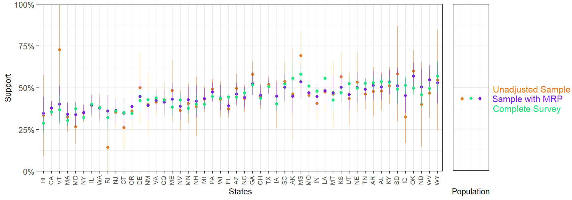
With a 5k sample, MRP lands much closer to the complete weighted survey than a 5k unweighted sample: neat. That’s certainly not a fully fair comparison, but it gives some intution around the promise of this approach.

Somewhat less neat is that even a 5k sample here takes about 13 minutes to fit. How does this change as we fit on more and more of the data?

Sample Size	Runtime
5,000	13 minutes
10,000	44 minutes
60,000	526 minutes (~8 hours!)

As the table above should illustrate, if you’re fitting a decently complex Bayesian model on even somewhat large N sizes, you’re pretty quickly going to cap out what you can reasonably fit in a acceptable amount of time. If you’re scaling N past the above example, or deepening the modeling complexity, you’ll pretty quickly feel effectively locked out of using these models in fast-paced environments.

Hopefully fitting my running example has helped for building intuition here. Even a reasonably complex Bayesian model can have some pretty desirable estimation properties. To make iterating on modelling choices faster, to scale our N or model complexity higher, or just to use a model like this day to day when time matters, we’d really like to scale these fitting times back. Can Variational Inference help?

Introducing Variational Inference

I’ve gotten relatively far in this post without clearly explaining what Variational Inference is, and why it might provide a more efficient and scalable way to fix large Bayesian models. Let’s fully flesh that out here to ground the rest of the series.

In the bigger picture, pretty much all of our efforts in Bayesian inference are a form of approximate inference. Almost no models we care about for real world applications have closed form solutions- conjugate prior type situations are a math problem for stats classes, not a general tool for inference.

Following Blei et al. (2018)’s notation, let’s setup the general problem first, describe (briefly) how MCMC solves it, and then more slowly demonstrate how VI does. Let’s say we have some observations x_{1:N}, and and some latent variables that define the model z_{1:M}. Note for concreteness these latent variables represent our quantities of interest: key parameters and so on- we’re calling them latent in the sense that we can’t go out and directly measure a \beta or \gamma from the model above, we have to gather data that allows us to estimate them. We call p(z) priors, and they define our model prior to contact with the data. The goal of Bayesian inference then is conditioning on our data in order to get the posterior:

p(z|x) = \frac{p(z,x)}{p(x)}

If you’re reading this post series, it’s likely you recognize that the denominator on the right here (often called the “evidence”) is the sticking point; the integral p(x) = \int{p(z,x)dz} won’t have a closed form solution.

When we use Markov Chain Monte Carlo as we did above to estimate the model, we’re defining a Markov Chain on z, whose stationary distribution if we’ve done everything right is p(z|x). There are better and worse ways to do this certainly- the development of the Stan language, with associated Hamiltonian Monte Carlo with NUTS sampler has massively expanded what was possible to fit in recent years. However, while actively improving the speed and scalability of sampling is an active area of research (for example, by using GPU compute where possible), some of the speed challenges just seem a bit baked into the approach. For example, the sequential nature of markov chains makes parallelization within chains seem out of reach absent some as-yet unknown clever tricks.

Instead of sampling, variational inference asks what we’d need to figure out to treat the Bayesian inference problem as an optimization problem, where we could bring to bear all the tools for efficient, scalable, and parallelizable optimization we have developed.

Let’s start with the idea of a family of approximate densities \mathscr{Q} over our latent variables⁵.

Within that \mathscr{Q}, we want to try the best q(z), call it q^*(z), that minimizes the Kullback-Leibler divergence to the true posterior:

q^*(z) = argmin_{q(z) \in \mathscr{Q}}(q(z)||p(z|x))

If we choose a good \mathscr{Q}, managing the complexity so that it includes a density close to p(z|x), without becoming too slow or impossible to optimize, this approach may provide a significant speed boost.

To start working with this approach though, there’s one major remaining problem. Do you see it in the equation above?

The ELBO

If you haven’t seen it yet, this quick substitution should clarify a potential issue with VI as I’ve described it so far:

q^*(z) = argmin_{q(z) \in \mathscr{Q}}(q(z)||\frac{p(z,x)}{\bf p(x)}) = \mathbb{E}[logq(z)] - \mathbb{E}[logp(z,x)] + {\bf logp(x)} Without some new trick, all I’ve said so far is to approximate a thing I can’t analytically calculate (the posterior, specially the issue evidence piece of it), I’m going to calculate the distance between my approximation and… the thing I said has a component can’t calculate?

Fortunately, a clever solution exists here that makes this strategy possible. Instead of trying to minimize the above KL divergence, we can optimize the alternative objective:

\mathbb{E}[logp(z,x)] - \mathbb{E}[logq(z)]

This is just the negative of the first two terms above, leaving aside the logp(x). Why can we treat maximizing this as minimizing the KL divergence? The logp(x) term is just a constant (with respect to q), so regardless of how we vary q, this will still be a valid alternative objective. We call this the Evidence Lower Bound (ELBO)⁶.

If it’s helpful for intuition, play around with this great interactive ELBO optimizer by Felix Köhler:

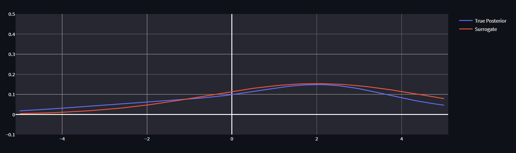
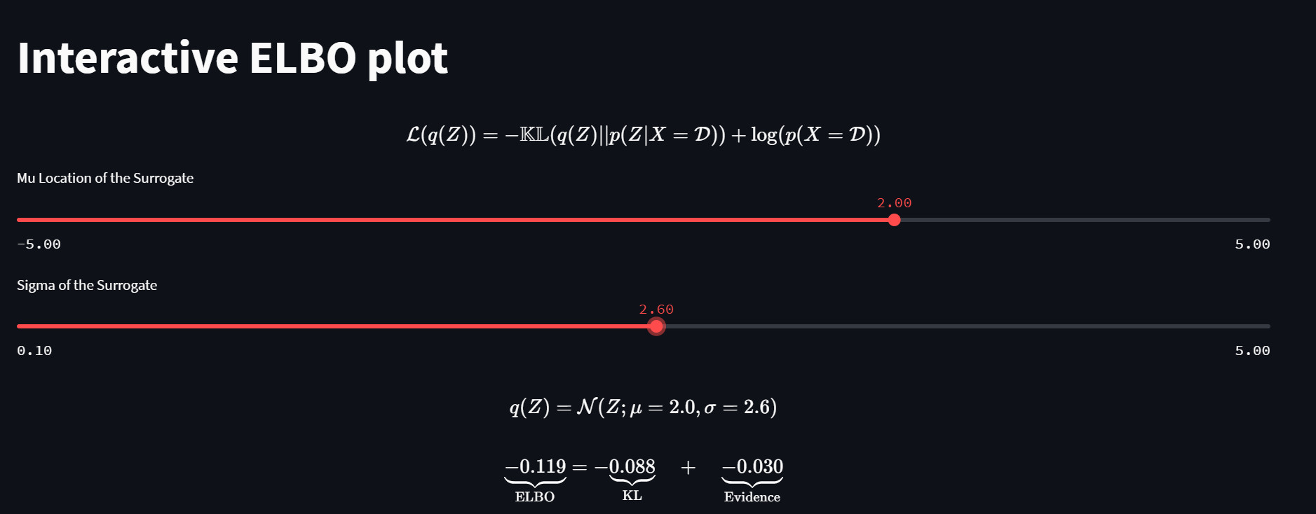
Link to demonstration here; check out Felix’s Youtube explanation of the ELBO also!

By twiddling the knobs on \mu and \sigma for our approximating normal, we can get our surrogate distribution pretty close to the True Posterior (which we know for purposes of demonstration, so we can calculate the true KL, not just it’s ELBO component). No matter how we twiddle though, the evidence remains constant.

For further intuition- notice that we can only do this trick in one direction. The KL divergence isn’t symmetrical, and if we wanted to calculate the “reverse” KL, we couldn’t use this strategy as logq(x) would not be a constant. Even if we thought that optimizing other direction of KL might have desirable properties like emphasizing mass-seeking over mode-seeking behavior, that simply isn’t an option.

A first try at VI on this dataset

Ok, so we have an objective to optimize that should actually work. What’s a good \mathscr{Q}? The choice has been shown to matter a lot, but for purposes of a first swing here, let’s try one of the simpler ideas people have explored, the mean-field family. These latent variables will be assumed mutually independent⁷ and each get it’s own distinct factor in the variational density. A member of this would look something like:

q(z) = \prod_{j=1}^{m} q_j(z_j)

Each latent z_j get it’s own variational factor with density q_j(z_j), whose knobs we play with to maximize the ELBO. In the particular implementation below normal distributions are used, plenty of other options like t distributions are common too.

Probably not the best we can do, but let’s give it a roll. Since we’ve been told this will scale really well too supposedly, let’s use all 60k of the observations just to get a sense how it’ll compare to our 8+ hours in that case.

tic()
fit_60k <- stan_glmer(abortion ~ (1 | state) + (1 | eth) + (1 | educ) + male +
                    (1 | male:eth) + (1 | educ:age) + (1 | educ:eth) +
                    repvote + factor(region),
  family = binomial(link = "logit"),
  data = cces_all_df,
  prior = normal(0, 1, autoscale = TRUE),
  prior_covariance = decov(scale = 0.50),
  adapt_delta = 0.99,
  refresh = 0,
  algorithm = "meanfield",
  seed = 605)
toc()

This finishes in a blazing 144.03 seconds. Is this a good fit, or have we created a ridiculous spherical cow?

You’ll have to find out in the next post. Thanks for reading!

Typically, I’ll include links to code at the end of these posts, but since the only thing going on in this notebook is mentioning some runtimes of the models displayed inline at various sample sizes, I’m skipping that for now.

Footnotes

If I were that type of Bayesian, this is where I’d complain that if we screw this up badly enough, we might as well be frequentists or worse, machine learning folk.↩︎
In grad school, using BART as the estimator (also combining it with some portions of the model being estimated as multilevel models) was the focus of my masters thesis. This pairs the best parts of relatively black box machine learning sensibility with the advantages of still having a truly Bayesian model. With comparatively minimal iteration you can get a pretty decent set of MRP models that will be better than many basic versions of multilevel models fit early in the MRP literature. Of course, if you’re willing to spend a bunch of time iterating on the absolute best models for a given problem, and incorporate lots of problem specific knowledge into model forms you can and should do better than BARP. Also, a lot of pretty cool things you can do like jointly model multiple question responses at the same time aren’t going to be easily to implement unless you get way in the weeds of your own BART implementation.↩︎
Insert snark about CCES folks doing a poor job at gender inclusivity despite 80+ researchers working on it here.↩︎
Again, see the MRP case studies linked above if you want see all the data prep and draw manipulation here; I’ll be leaving out most such details that aren’t relevant for comparisons to fitting this model with VI from now on.↩︎
In grad school, I had a friend who insisted on calling this “spicy Q”. For a while we had a latex package that made \spicy{} equivalent to \mathscr{}. Apologies for the footnote for the dumb LaTeX joke, but now I’m pretty sure you won’t have a sudden moment of “what is that symbol again” discussing VI ever.↩︎
Why is this a lower bound? Notice that we could write the evidence from above equations as logp(x) = KL(q(z)||p(z|x)) + ELBO(q). Since the KL divergence is non-negative (it’s zero when distributions p and q are identical), the ELBO is a lower bound of the evidence.↩︎
If this seems like it could go fully spherical cow, both literally in the sense that if we use a bunch of independent normals we make a sphere, and in the sense that this may not represent the full complexity of public opinion, you’re correct. Assuming independence here could very easily cause problems, and part of why this VI strategy is so challenging is the subset of things we can easily optimize doesn’t have the best overlap with fully realistic distributional assumptions over our latent variables.↩︎

Reuse

https://creativecommons.org/licenses/by/4.0/

Citation

BibTeX citation:

@online{timm2022,
  author = {Andy Timm},
  title = {Variational {Inference} for {MRP} with {Reliable} {Posterior}
    {Distributions}},
  date = {2022-10-10},
  url = {https://andytimm.github.io/variational_mrp_pt1.html},
  langid = {en}
}

For attribution, please cite this work as:

Andy Timm. 2022. “Variational Inference for MRP with Reliable Posterior Distributions.” October 10, 2022. https://andytimm.github.io/variational_mrp_pt1.html.