This post is a brief introduction to nutpieR’s new “Bring Your Own Density Kernel” feature. I’m using density kernel to refer to a shared library that computes a Stan model’s unconstrained log density and full gradient.1 It replaces BridgeStan’s density evaluation in the larger sampling loop; the usage of the nuts-rs sampler is unchanged.
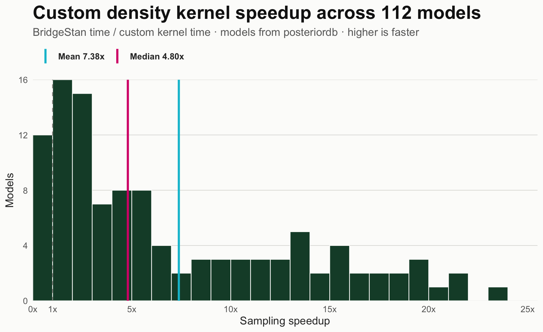
Supplying your own density kernel is easier than it sounds, and provides a 4.8x median (7.4x average) speedup compared to vanilla nutpieR sampling in my testing across 112 posteriordb models.
The first part of this post introduces the notion of bringing your own log density evaluator and nutpieR API for doing so, and the second uses the posteriordb benchmarking run mentioned above to build intuition on how these speed gains are realized.
This feature allows users to supply their own density and gradient evaluation code, typically written in Rust or C++, and otherwise sample as normal via nutpieR. The model itself remains written in Stan, and the sampling algorithm remains the same nuts-rs sampler the package wraps.
I’ll discuss performance in more depth later, but in brief, custom evaluators have the potential for several times speedups because they can be written to be highly model specific. In contrast, while the Stan autodiff is truly wonderful, its stunning generality necessarily comes at a performance price. If we just need to define a kernel for a single model (with possibly fixed data), we can expect to be able to often do better.
In some sense, custom kernels like this have always been an option if you had a single Bayesian model you really, really wanted to make faster, but recent improvements in LLM coding capacity have made choosing to build model specific evaluators significantly more realistic and accessible. This is a near idealized task for a coding model given the clean evaluation loop: we can give an LLM an oracle function (the Stan density and gradient evaluators), insist that a proposed kernel match Stan to within tolerance to be considered valid, while hillclimbing on speed and memory efficiency. A great project, Alchemize, aims to systematize this idea of ‘LLM Transpilation’ into an easy to use agent loop.
Interface
The nutpieR interface exposes 3 slim functions to make validating and sampling from models with your own log density easy.
To make things more concrete, let’s step through optimizing a simplistic regression model:
Let’s first fit it with nutpieR using the default, built-in BridgeStan density and gradient components to get a baseline speed:
library(nutpieR)library(posterior)# Basic DGPN <-1000x <-seq(-2, 2, length.out = N)y <-1.25-0.7* x +0.6*sin(seq_len(N) *1.61803398875) +0.15*cos(seq_len(N) *0.37)data <-list(N = N, x = x, y = y)reference <-nutpie_compile_model("linear.stan")settings <-list(num_draws =10000,num_warmup =400,num_chains =4,cores =4,progress ="none",refresh =0)fit_reference <-do.call( nutpie_sample,c(list(model = reference, data = data, seed =604), settings))attr(fit_reference, "sampling_time")
[1] 0.343
To build a custom density kernel for this problem, we first need to understand the shape of the object nutpieR expects back from the kernel for a given model. We can use nutpie_density_layout() to clarify this:
At this point, I’d emphasize that if lower level languages like Rust/C++ aren’t your thing, the process of writing a kernel to this spec and validating it are relatively easy tasks for your friendly local LLM. More on that type of workflow in the next section.
The model here is pretty simple, so it shouldn’t be too hard to interpret what we’re expected to return. The kernel gets a three-element vector in the exact order alpha, beta, then the unconstrained value of sigma. Because sigma is lower-bounded, that third value is actually log(sigma); the kernel needs to transform it and include the lower-bound Jacobian. The layout string joins the same raw BridgeStan names with newlines and has no trailing newline.
Giving GPT-5.6 Terra2 a quick prompt with the above + access to the nutpieR docs gets us back the following kernel in a couple minutes:
That’s the interesting part of the kernel. The full source also handles the runtime JSON data and implements the other functions required by the ABI.
While recent LLMs are pretty good about the whole “make sure the kernel works” thing, we can further kick the tires with nutpie_validate_density_kernel(), which validates the shape of the returned log density and gradient evaluations, and compares a small set of points to BridgeStan to ensure they match within tolerance.
Treat this checker as a reasonable form of kicking the tires, but keep in mind that you’re ultimately responsible for validating the kernel you bring. For example, the package isn’t aiming to fully check equivalence in all the relevant parts of posterior space (that’s hard to know in a model agnostic sense), or protect you from “creative” kernels that may match at a handful of points but aren’t fully memory safe, or might crash your R session. The function here is defined to give you reasonable peace of mind, not replace validation during kernel building.
# The kernel was compiled into library path right before this step;# code for that isn't that interesting.bound <-nutpie_attach_density_kernel(reference, library_path, data = data)random_check <-nutpie_validate_density_kernel( bound, seed =604, num_points =100)# You can also sample n points from a regular BridgeStan reference trajectory to get a slightly more realistic set of pointsreference_check <-nutpie_validate_density_kernel( bound, seed =604, num_points =100, method ="reference")print(random_check)
Density kernel check: pass (advisory); points: 104 pass, 0 fail, 0 inconclusive
  reference: 100 points; pointwise pass (100 pass, 0 fail, 0 inconclusive)
  random: 4 points; pointwise pass (4 pass, 0 fail, 0 inconclusive)
Reference pilot: 1 chain, 200 warmup + 100 draws; 0.011 s (BridgeStan only)
Pilot diagnostics: $pilot$diagnostics; short pilot is not a convergence guarantee.
Max absolute difference: logp 7.28e-12; gradient 5.82e-11
Repeatability: pass (q1, q2, q1)
Details: $comparisons, $gradients, $repeatability, $tolerances, $untested
All looks well here. In cases where the kernel doesn’t meet expectations, the function provides helpful feedback on the shape or calculation disagreements that it found for use in further improvements.
Now for the fun part! Let’s sample with the new kernel and see if we’ve achieved much of a speedup:
Show timing and comparison setup
# Warm both paths outside the timer.invisible(nutpie_sample( reference, data = data, num_draws =100, num_warmup =100,num_chains =2, cores =2, seed =900, progress ="none"))invisible(nutpie_sample( bound, num_draws =100, num_warmup =100,num_chains =2, cores =2, seed =900, progress ="none"))rows <-list()last_fit <-list()for (i in1:3) { seed <-604+ i methods <-if (i %%2) {c("bridgestan", "kernel") } else {c("kernel", "bridgestan") }for (method in methods) {gc() elapsed <-system.time({ fit <-if (method =="bridgestan") {do.call( nutpie_sample,c(list(model = reference, data = data, seed = seed), settings) ) } else {do.call( nutpie_sample,c(list(model = bound, seed = seed), settings) ) } })[["elapsed"]] diagnostics <-nutpie_diagnostics(fit) rows[[length(rows) +1]] <-data.frame(rep = i,method = method,elapsed = elapsed,divergences =sum(diagnostics$diverging),maxdepth =sum(diagnostics$maxdepth_reached) ) last_fit[[method]] <- fit }}timings <-do.call(rbind, rows)medians <-aggregate(elapsed ~ method, timings, median)speedup <- medians$elapsed[medians$method =="bridgestan"] / medians$elapsed[medians$method =="kernel"]summary_columns <-c("mean", "sd", "rhat", "ess_bulk")reference_summary <-as.matrix(summarise_draws(last_fit$bridgestan)[summary_columns])kernel_summary <-as.matrix(summarise_draws(last_fit$kernel)[summary_columns])comparison <-all.equal( reference_summary, kernel_summary,# This might be a bit overkill for more complex models but for a simple model it's safetolerance =1e-6,check.attributes =FALSE)# Just sanity check the results are equivalentif (!isTRUE(comparison)) print(comparison)stopifnot(isTRUE(comparison))
Sick, 6.23x faster, with matching posterior summaries!
I’ll talk more generally about ‘causes’ of speedup in the next section, but if it’s helpful early intuition, squinting at the kernel above, most of what’s likely going on here is a custom kernel sidestepping the necessary autodiff in BridgeStan’s more general solution through the Stan math library. There may be some minor gains as well from operator fusion– the kernel calculates the likelihood and all three gradient contributions in one pass over the data, reusing each residual – but for something so simple most gains will be the generic “having to do less work” by routing around autodiff.
In this case of course, this model was already plenty fast, but this form of purely computational gain (no sampler algorithm change here) remains feasible for far more complex models.
Kernel design with LLMs
Before I share a less “hello world” benchmark of this approach, let’s talk about working with LLMs to build these kernels, and how this feature’s design anticipates LLMs typically being in the loop here.
Here’s the prompt I used to request the simple kernel above:
Show prompt
Test a minimal Gaussian linear regression with a custom nutpieR density kernel
end to end. Work only in a scratch directory and leave the package repository
untouched.

Use the Stan model and deterministic N = 1000 data above. Read the installed
kernel-writing guide and nutpier_density_kernel_v1.h header before implementing
anything. Build a small C shared library with runtime JSON data binding and the
exact layout returned by nutpie_density_layout(). Match BridgeStan's
propto = TRUE, jacobian = TRUE target, including sigma = exp(raw_sigma), its
Jacobian, and the full analytic gradient. Alchemize can be optimization
inspiration, but follow nutpieR's ABI and lifecycle contract.

Compile the library with R CMD SHLIB and attach it with
nutpie_attach_density_kernel(). Run both the default random check and
nutpie_validate_density_kernel(..., method = "reference") without loosening
tolerances. Then run a short sampling smoke test. Report the compiler command,
validation output, assumptions, and any remaining risks. Do not treat the
numerical checker as proof of memory or thread safety.
Relatively simple, right? The prompt for the broader benchmark below is only slightly more complex (mostly to generalize it to the multiple task and constrain the level of effort I wanted). You truly don’t need a ton of initial detail to get an agent going smoothly in the right direction here, given how verifiable and closed this task loop is.
I decided against including any more substantial prompting/validation scaffolding like Alchemize provides, both because Alchemize already exists and is great3, but also because a prompt like the above is already pretty much sufficient with current models. Instead, I’ve mostly focused on providing tools for LLMs (and their users) to understand what’s expected of a density kernel, and validate that kernel is correct.
Beyond some of the functions anticipating LLMs as primary users, one more awkward part of this is how to handle documentation. In this case, while things like the main package README and function docs remain more firmly focused on the human reader, the primary jumping off point for building a kernel, inst/examples/density-kernel/README.md, is optimized more heavily for LLM consumption4.
Writing this sort of “mixed audience” software and documentation in 2026 is rather weird, but hopefully I’ve struck a decent balance.
Benchmarking for fun and intuition
To validate the feature and get a better understanding of available gains, I made relatively basic kernels for 112 models5 from posteriordb. All of these kernels were validated to match BridgeStan density and gradient evaluations, and I compared resulting samples for reasonable equivalence to vanilla nutpieR6. All of the example kernels and a bit more detail can be found here.
To give a rough sense of implementation quality, I’d characterize these kernels as pretty reasonable first passes- I explicitly prompted the implementing agents to get something reasonable working without spending too much time hillclimbing. Most kernels ended up taking a couple minutes to draft and were well-validated within 15 minutes. That said, a few harder models took several additional passes either to fix initial correctness issues (caught with the diagnostic function) or to implement more involved models. I also constrained the models to use the original data shape and model form, so that the speedup measured is fairly purely just about the density kernel differences7.
On average, the speed gains are pretty substantial:
Measurement
Mean speedup (BridgeStan / custom kernel)
Median speedup (BridgeStan / custom kernel)
Custom kernel faster
NUTS sampling wall time
7.38x
4.80x
100/112
Log density + full gradient
10.15x
8.74x
99/112
Visually:
radon_all-radon_pooled is a 49.6x result outside the plotted range; it remains included in the mean and median.
If you’re curious about particular models, the model-level median sampling times and ratios behind the table and figure are available as a small CSV.
Qualitatively, where’s the speed come from?
The other nice thing about running a benchmark like this is we can survey the techniques agents used. Without claiming this is an exhaustive list of tricks, a reasonable group level summary is something like:
Sidestepping autodiff: Autodiff is incredible, and helps keep the Bayesian iterative workflow sane, but being able to return a gradient directly without Stan Math’s autodiff runtime is a huge boon for speed. Almost every model here was able to avoid any form of AD via manually specified derivatives.
Problem specific structure: Many problems have specific structure that enables custom operations or data structures that are more efficient. One simple example is in hierarchical models, where each observation can accumulate its contribution directly into the relevant group’s gradient entry. All manner of little problem specific tricks like this are sprinkled throughout the kernels, and there are probably more that could be integrated in with more effort.
Operator Fusion: Operator Fusion combines sequential operations into one; for example, the regression kernel above calculates each residual once, then accumulates everything needed for the likelihood and all three gradient terms in the same pass over the data.
Minimizing Data Movement: Avoiding unneeded data movement and allocations can add up. Only needing to support one model allows the kernels to do things like efficiently reuse temporary storage and avoid reallocation.
The 12 places where these initial kernels aren’t faster in sampling are also informative. The slowest by far is a Gaussian process (state_wide_presidential_votes-hierarchical_gp), where Stan ships a clever Eigen-backed Cholesky thing, and many of the others are largely regressions using the very well optimized bernoulli_logit_glm_lpmf and normal_id_glm_lpdf functions from Stan. It might be possible to do better than these with more effort, but I thought it’d be more realistic to include some cases where a novel kernel doesn’t win.
More granularly adjudicating how much each bucket of tweaks is worth would require more comparisons than I want for a feature release post. That said, the broader design space looks pretty promising if you’re willing to put a reasonable amount of (LLM-assisted) work into a specific problem. Even if a model doesn’t have useful structure Stan Math wasn’t able to exploit, many real models can at least benefit meaningfully from replacing autodiff with specific solutions, for example.
Conclusions
Hopefully this post has gotten you interested in bringing your own density kernel to nutpieR! I’m hopeful it’ll allow you to more quickly build and fit ambitious models.
This work was heavily inspired by PyMC Labs’ great work on Alchemize, and how python nutpie integrates the sampler with custom densities and gradients. The Alchemize blog post linked is a really great next read here on the use of LLMs to build your own kernels. I’ve also been inspired by Blackjax’s work towards a significantly more modular system for Bayesian inference in composing sampler algorithm components, and the remarkable amount of optimization pressure applied to GPU kernels for LLM training and serving.
A note on AI writing and this blog: All of the writing/editing of this post is my own. The orchestration of the larger posteriordb benchmark, example kernels themselves, repo packaging of that benchmark, along with much of the feature implementation heavily lean on agentic support, primarily via prime-agent running recent OAI models. Of course, more broadly, my view is I’m responsible for the correctness, honesty, and legibility of the broader project and feature regardless of any level of LLM usage throughout.
Footnotes
I waffled a decent bit on what name to use for this. Kernel is a bit overloaded as a term (MCMC transition kernels, Covariance Kernels for GPs, and GPU kernels are all things…), but it felt useful as a gesture at this being a computational tool for the density + gradients. Something like “log-density evaluator” or “target evaluator” also could work, but didn’t feel like they pointed towards this being primarily computational as much. Names are the hardest problem in software engineering, part 1713.↩︎
You can absolutely use weaker LLMs for this type of task, especially for a kernel this simple. Conversely, if you’re aiming to squeeze out every last drop of performance, going bigger can make sense.↩︎
This is a good place to note that what Alchemize aims to output and what nutpieR wants from a density kernel aren’t exactly equivalent given the slightly different project goals. I’ve aimed to keep them similar enough that an LLM building a kernel can look to Alchemize for inspiration.↩︎
If you’re curious what “optimized for LLM consumption” means in practice, I largely experience this as lowering but not voiding my standards for prose and organization of information for human readers. I also asked agents rolling a kernel in the posteriordb benchmark I discuss later to leave notes about any common gotchas, confusions, or wishlist documentation they requested, and (had an agent) read through and integrate those into the README.↩︎
I started with the 114 models used in Seyboldt, Carlson, and Carpenter’s preconditioning paper, then excluded two ODE models that’d be relatively more annoying to write a decent kernel for.↩︎
Most of these cases are pretty straightforward to verify reasonable equivalence of posterior means, SDs, diagnostics, etc. In the interest of being transparent though, some of the models that mixed poorly in both cases like bball_drive_event_0-hmm_drive_0 and three_men2-ldaK2 are a little ambiguous: what does it mean to “reasonably match” a somewhat unstable posterior estimate?↩︎
For example, some of the problems could’ve benefited from a sufficient statistic approach to boil down their inputs, but that doesn’t really feel in the spirit of the challenge so I wanted to rule that out.↩︎